Flying Drone DIY, part V: custom autopilot programs -- improving computer vision of drone
Executive summary
Innovative custom solution for driving drone over optical flow gave first satisfactory results. The next steps would be to continue improve this approach and remove april tags from optical flow that were additional support for algorithm navigation.
At the previous step standard OpenCV solutions, ML and hybrid solutions didn't give satisfactory results. Next idea was to make an attempt to solve the task by extracting all possible features from the images, estimate their changes, rank them and apply superset of their input according to the significance.
Results of this R&D work are working visual recognition pipeline which transform optical flow into driving commands to the drone with acceptable level of correctness.
Tech stack:
Python, MAVSdk, Gazebo, Computer Vision
Research & development
Straightforward approach to solve image recognition and flight stabilization issues didn't work out: it recognize the markers and respond by tunning engines, but it does it in a way that a bit far from what is expected.
Going deep to the root cause shown homography of the image doesn't give clear signal, clear enough to drive a drone. Improving homorgraphy results seems as a dead end and I started to search for alternative approaches.
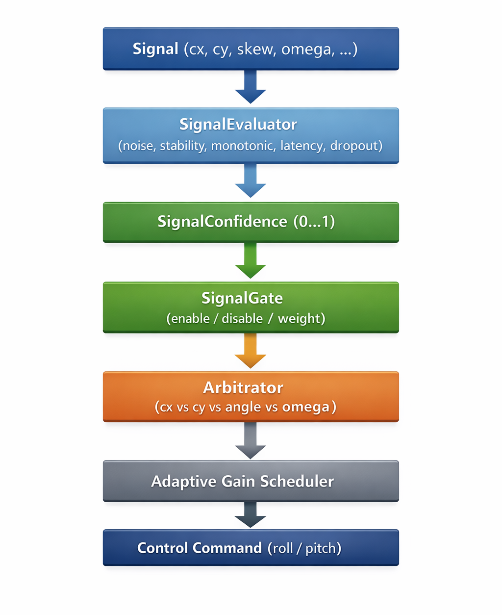
Such alternative approach is to extract several features of the image and to use result of their analysis as a potential signal for a drone maneuvering. Such signals goes over evaluation pipeline which filtrates weak and noisy signals and ended up with a short list of signals which are allowed to drive a drone.
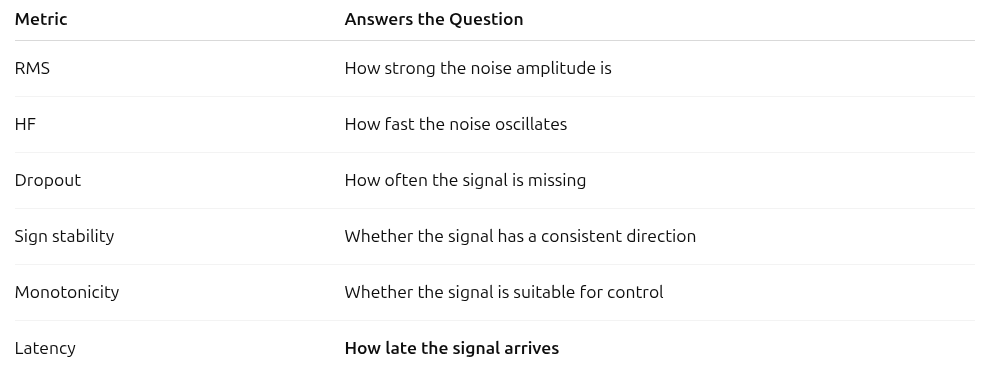
Features of the image
What we can take from the image for analysis? Here is a short
list of features:
- Center of the marker
- Axis of the marker
- Aspect of the marker
- Skew of the marker
- How fast the marker moves -- speed
- How fast the marker rotates -- rotation speed
Signal analysis
All these metrics are computed in real time inside SignalEvaluator and ConfidenceLayer classes.
RMS of noise
This metric is useful to understand can we rely on this signal for controlling the drone. RMS measures the average deviation of the signal from its local trend (EMA), serving as a practical estimate of noise magnitude.dispersion how far varies signal from its expected normal curve. Such variations are possible a noise. High value means we can't use it for drone control. Low value means we can rely on it.
                    def prepare_rms_of_noise(self, ema_window=10):

                        def rms(signal):
                            if not self.signal_filter.allows(signal.name, SignalMetricsNames.NOISE):
                                raise Exception(f'RMS doesn\'t support {signal.name}')

                            self.buffer.update(signal)
                            values = np.array(self.buffer.values(signal.name))

                            if len(values) < ema_window:
                                return None

                            ema = np.convolve(
                                values,
                                np.ones(ema_window) / ema_window,
                                mode="same"
                            )

                            return float(np.sqrt(np.mean((values - ema) ** 2)))

                        return rms
ema_window controls locality
Larger window → slower trend → higher RMS
Smaller window → more aggressive jitter detection
RMS noise can be thresholded qualitatively and safely today using normalized bands, but any absolute “valid / invalid” cutoff requires observing the drone in closed loop.
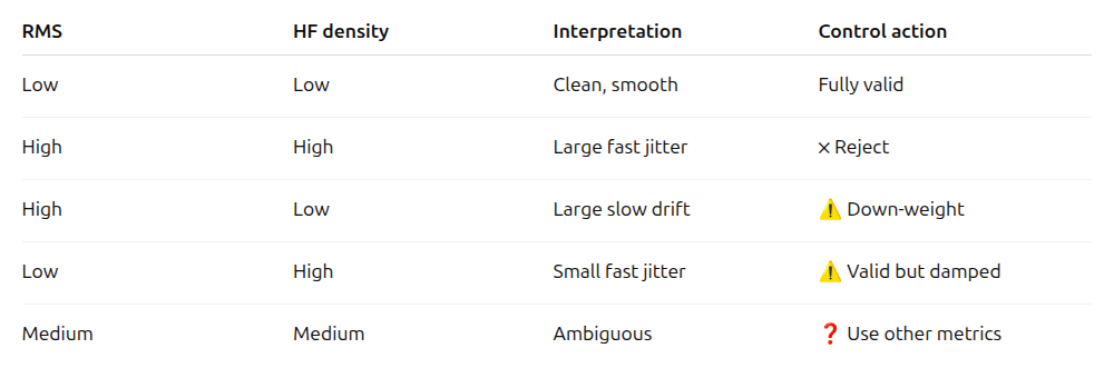
Spectral density and high frequency spectral density
Spectral density estimates how rapidly the signal varies, while RMS estimates how large those variations are. A signal should be rejected only when both variation magnitude and variation speed are high. Low RMS with high HF indicates small but fast jitter and should be handled by gain reduction rather than rejection, while moderate values in both metrics require additional context to determine validity.
This metric is not a physically normalized power spectral density. It is a heuristic frequency-domain indicator intended for relative comparison between signals.
                    def prepare_spectral_density(self):

                        def spectral(signal):
                            self.buffer.update(signal)
                            values = np.array(self.buffer.values(signal.name))

                            if len(values) < 8:
                                return None

                            fft = np.fft.rfft(values - np.mean(values))
                            power = np.abs(fft) ** 2

                            # part of the energy in HF
                            hf = power[len(power)//2:]
                            return float(np.mean(hf))

                        return spectral
Dropout rate
This metric estimates how often signal samples are missing or delayed. The signal is treated as a time-ordered sequence, and gaps between consecutive timestamps are analyzed. If the time gap between samples exceeds the expected update interval, it is counted as a dropout. A high dropout rate indicates unreliable temporal continuity and reduces the signal’s suitability for analysis and control.
                    def prepare_dropout_rate(self, expected_dt):

                        def dropout(signal):
                            self.buffer.update(signal)
                            ts = self.buffer.timestamps(signal.name)

                            if len(ts) < 2:
                                return 0.0

                            gaps = np.diff(ts)
                            dropouts = gaps > (1.5 * expected_dt)

                            return float(np.mean(dropouts))

                        return dropout
Dropout rate does not capture delayed but continuous signals — this is intentionally handled by latency.
Sign stability of signal
Sign stability measures the consistency of the signal’s directional polarity over time. Frequent sign changes indicate loss of directional meaning, oscillatory behavior, or unreliable estimation, making the signal unsuitable for direct control.
cx / cy -- determines the direction of correction
angle -- determines the side of the slope
omega -- determines the direction of rotation
                    def prepare_sign_stability(self):

                        def stability(signal):
                            self.buffer.update(signal)
                            values = np.array(self.buffer.values(signal.name))

                            if len(values) < 3:
                                return None

                            signs = np.sign(values)
                            signs = signs[signs != 0]

                            if len(signs) == 0:
                                return 0.0

                            return float(abs(np.sum(signs)) / len(signs))

                        return stability
Sign stability does not measure accuracy — it measures directional consistency.
Latency of the signal
Latency here is used not for analysis of the signal, but for
decision making. Code doesn't measure the gap since an event
occurrence, but time gape since the most significant change in
the signal.
This is not an absolute sensor-to-actuator latency, but a
relative responsiveness estimate.
Signal Arbitration (Most Important)
When multiple signals are available:
- cx (position)
- angle (tilt)
- omega (angular velocity)
and all of them are considered correct, but have different latencies, the rule is simple:
lower latency → higher priority
This is a classical control principle: a less accurate but fast signal is often preferable to a highly accurate but delayed one.
Therefore, latency becomes a key weighting factor in the Arbitrator.
Adaptive Gain Scheduling
Signal delay increases phase shift in a closed-loop system.
As latency grows:
- reduce controller gain
- increase damping
Even a rough latency estimate can significantly reduce the risk of oscillations and instability.
Detection of “Stale” Signals
Computer vision pipelines often produce:
- irregular updates
- burst-like outputs
Latency helps detect cases where:
- the signal is technically alive, but outdated
- the signal has not dropped out (
dropout = 0), yet is no longer usefulThis represents a separate dimension of signal assessment, orthogonal to dropout.
Channel Desynchronization Filtering
Example:
- cx responds quickly
- angle responds slowly
Possible causes include:
- pipeline lag
- buffering effects
- internal branching in the CV pipeline
Latency analysis helps:
- detect channel desynchronization
- reduce trust in slower channels
                    def prepare_latency(self):

                        def latency(signal):
                            self.buffer.update(signal)
                            values = np.array(self.buffer.values(signal.name))
                            ts = np.array(self.buffer.timestamps(signal.name))

                            if len(values) < 5:
                                return None

                            dv = np.diff(values)
                            idx = np.argmax(np.abs(dv))

                            if idx <= 0 or idx >= len(ts):
                                return None

                            return float(ts[-1] - ts[idx])

                        return latency
Monotonic signal
Monotonicity measures whether a signal changes consistently in one direction and can be safely used as a control input rather than a noise-driven measurement.
Monotonicity may temporarily drop during legitimate oscillatory dynamics (e.g., hover stabilization), therefore it should be interpreted in context and combined with other metrics rather than used as a hard gate.
Protection against “false control”
Computer vision signals often:
- Oscillate around the true value
- Suffer from quantization effects
- “Reinterpret” the scene over time
This signal will not drive the drone back and forth, even if it is numerically accurate.
Monotonicity expresses exactly this property.
Weight in the Arbitrator
If:
- RMS is acceptable
- HF energy is acceptable
- Dropout rate is zero
- Latency is low
but:
- Monotonicity is low
The signal should lose arbitration to a coarser but directionally consistent signal.
Adaptive gain scheduling
Low monotonicity implies:
- Reducing control gain
- Increasing damping
- Disabling the integrator
This is a direct protection mechanism against self-excitation.
                    def prepare_monotonic_coefficient(self):

                        def monotonic(signal):
                            self.buffer.update(signal)
                            values = np.array(self.buffer.values(signal.name))

                            if len(values) < 3:
                                return None

                            diffs = np.diff(values)
                            signs = np.sign(diffs)
                            non_zero = signs[signs != 0]

                            if len(non_zero) == 0:
                                return 0.0

                            # 1.0 → строго монотонно
                            # ≈0 → шум / колебания

                            return float(abs(np.sum(non_zero)) / len(non_zero))

                        return monotonic
Can we trust this signal?
The next step is to understand could we really rely on this signal for a drone control. Each signal's metric has corresponding weight which is multiplied on value of the signal: in this case the most important metrics count more and less important metrics count less. It works as a filter.
                    weights={
                        SignalMetricsNames.STABILITY:         0.25,
                        SignalMetricsNames.NOISE_RMS:         0.20,
                        SignalMetricsNames.NOISE_STD:         0.20,
                        SignalMetricsNames.MONOTONIC:         0.15,
                        SignalMetricsNames.DROPOUT_RATE:      0.15,
                        SignalMetricsNames.LATENCY:           0.15,
                    })

                    if metrics.rms_noise is not None:
                        self._assert_normalized(metrics.rms_noise, SignalMetricsNames.NOISE_RMS)
                        score = 1.0 - metrics.rms_noise
                        self._add_score(
                            weighted_scores,
                            SignalMetricsNames.NOISE_RMS,
                            score
                        )
How does such has been chosen? Based on empirical knowledge gathered over AI. It is just a start point then this weight should be tuned further based on new data.
Not all metrics are applied to each signal. Therefore the weight of each metric will be increased in the not completed signal's weight vector. It is done over normalization at the end of the method.
                    total_weight = sum(w for w, _ in weighted_scores)

                    if total_weight <= 0.0:
                        return 0.0

                    return sum(w * s for w, s in weighted_scores) / total_weight
Choosing the right signal
At this stage the system already knows the reliability of every signal. The question is: which ones should actually drive the drone right now?
We solve this with a two-level arbitration system:
- SignalGate — quickly discards clearly bad channels using hysteresis and minimum stability time.
- Arbitrator — makes the final decision with the following priority:
- Both
IMAGE_X+IMAGE_Yare confident → use both (highest accuracy) - One of them dropped below threshold → fallback to the remaining strong channel (single-channel mode)
- Neither position channel is usable → try
ANGLE - Still nothing → try
OMEGA - Nothing works → HOLD (0, 0, 0, 0)
This fallback mechanism is the key improvement of version V2. The drone no longer freezes when one axis temporarily loses the marker — it continues flying on the remaining reliable channel.
Convert signal into drone drive command
The final stage is transforming the selected and weighted signals into control commands.
After applying speed limiting, and possible compensation (e.g., when using only one channel), the command is sent via MAVLink to PX4. The loop is closed.
At this point we have a fully functional vision-based control system using AprilTag with reasonably high robustness to noise, vibration, and short-term marker loss.
Results & Flight Behaviour
With the loose configuration and single-channel fallback the drone now:
- Stably holds position when the marker is well visible
- Continues controlled flight even when one axis temporarily drops below threshold
- Shows smooth transitions between BOTH → single-channel modes
- Does not oscillate or run away (thanks to adaptive gain scheduling)
Video demonstration (Gazebo):
Conclusion
We now have a robust, explainable, and fully custom optical-flow controller that works reliably even under imperfect conditions. The combination of per-signal metrics, intelligent gating, and fallback arbitration turned a previously unstable idea into a working autopilot component.
Next steps:
- Fine-tuning confidence weights and gating thresholds
- Adding motion prediction (Kalman filter or simple extrapolation)
- Moving to more challenging conditions: low light, fast rotations, partial occlusions
- Integration with other sensors (LiDAR, IMU fusion)
A few related publications:
Flying Drone DIY, Part IV: custom autopilot programs
Flying Drone DIY, Part III: Assembling and Tuning
Flying drone DIY, part II: configuration for the 1st version
Flying drone DIY, part I: discovery phase